Implementing Poincaré Embeddings in PyTorch

24 Jul 2020

After having introduced Riemannian SGD in the last blog post, here I will give a concrete application for this optimization method. Poincaré embeddings [1][2] are hierarchical word embeddings which map integer-encoded words to the hyperbolic space.

Even though the original paper used the Poincaré unit ball, any reasonable manifold can work. For example, when the data is not really a tree, the Euclidean space can produce better embeddings.

Poincaré Embeddings consist of the following components:

• dataset: \(\{(w_1, v_2), \dots, (w_n, v_n)\}\) where \(w_i\) is the parent and \(v_i\) is the child (e.g. hypernym and hyponym)
• distance function: the Poincaré ball needs \(d(x, y) = \text{arcosh}\left(1 + 2\frac{\lvert\lvert x - y\rvert\rvert^2}{(1 - \lvert\lvert x\rvert\rvert^2)(1 - \lvert\lvert y\rvert\rvert^2)}\right)\), while the Euclidean space uses \(d(x, y) = \lVert x - y\rVert_2^2\)
• loss function: \(\log\left(\text{softmax}\left(-d(x, y)\right)\right)\) (“categorical crossentropy”)
• weights: a single \(m \times n\) matrix where \(m\) is the input vocabulary and \(n\) is the output vocabulary (projection)
• metric: words that are neighbors should be closer together in a ranking than words that have no connection (“mean rank”).

Implementation

Model

First, we create the weights using the function Embedding. Then they are initialized close to \(0\). Since the Poincaré ball requires \(\lvert\lvert x\rvert\rvert < 1\), this won’t cause any trouble.

During forward propagation the input is split into two parts: parent (0 to 1) and children (1 to n). Next, we compute the distance between all nodes.

class Model(torch.nn.Module):
    def __init__(self, dim, size, init_weights=1e-3, epsilon=1e-7):
        super().__init__()
        self.embedding = Embedding(size, dim, sparse=False)
        self.embedding.weight.data.uniform_(-init_weights, init_weights)
        self.epsilon = epsilon

    def dist(self, u, v):
        sqdist = torch.sum((u - v) ** 2, dim=-1)
        squnorm = torch.sum(u ** 2, dim=-1)
        sqvnorm = torch.sum(v ** 2, dim=-1)
        x = 1 + 2 * sqdist / ((1 - squnorm) * (1 - sqvnorm)) + self.epsilon
        z = torch.sqrt(x ** 2 - 1)
        return torch.log(x + z)

    def forward(self, inputs):
        e = self.embedding(inputs)
        o = e.narrow(dim=1, start=1, length=e.size(1) - 1)
        s = e.narrow(dim=1, start=0, length=1).expand_as(o)

        return self.dist(s, o)

The line x = 1 + 2 * sqdist / ((1 - squnorm) * (1 - sqvnorm)) causes numerical instability. When using double-precision floating-point, epsilon can often be set to \(0\).

Training

First, set torch.set_default_dtype(torch.float64). This is not strictly necessary, but gives slightly better results and makes the network more stable.

Next, we need two distributions:

• categorical distribution: during the first \(20\) epochs, words/relations that occur more often are drawn with a higher frequency.
• uniform distribution: every word/relation has the same chance of being drawn.

It is not mentioned in the original paper, but the offical code follows this approach.

cat_dist = Categorical(probs=torch.from_numpy(weights))
unif_dist = Categorical(probs=torch.ones(len(names),) / len(names))

model = Model(dim=DIMENSIONS, size=len(names))
optimizer = RiemannianSGD(model.parameters())

loss_func = CrossEntropyLoss()
batch_X = torch.zeros(10, NEG_SAMPLES + 2, dtype=torch.long)
batch_y = torch.zeros(10, dtype=torch.long)

while True:
    if epoch < 20:
        lr = 0.003
        sampler = cat_dist
    else:
        lr = 0.3
        sampler = unif_dist

    perm = torch.randperm(dataset.size(0))
    dataset_rnd = dataset[perm]
    for i in tqdm(range(0, dataset.size(0) - dataset.size(0) % 10, 10)):
        batch_X[:,:2] = dataset_rnd[i : i + 10]

        for j in range(10):
            a = set(sampler.sample([2 * NEG_SAMPLES]).numpy())
            negatives = list(a - (set(neighbors[batch_X[j, 0]]) | set(neighbors[batch_X[j, 1]])))
            batch_X[j, 2 : len(negatives)+2] = torch.LongTensor(negatives[:NEG_SAMPLES])

        optimizer.zero_grad()
        preds = model(batch_X)

        loss = loss_func(preds.neg(), batch_y)
        loss.backward()
        optimizer.step(lr=lr)

Note only the first two words in batch_X are real relations. All other words are randomly drawn from either the uniform or categorical distribution. The ground truth for CrossEntropyLoss is always the first element batch_y = torch.zeros(10, dtype=torch.long). All other children are negatives.

Visualizations

After having trained the neural network, we can visualize our embeddings.

import matplotlib.pyplot as plt

model = torch.load("poincare_model_dim_2.pt")
coordinates = model["state_dict"]["embedding.weight"].numpy()

plt.xlim(-1, 1)
plt.ylim(-1, 1)
plt.axis('off')

for x in range(coordinates.shape[0]):
    plt.annotate(model["names"][x], (coordinates[x,0], coordinates[x,1]),
                 bbox={"fc":"white", "alpha":0.9})

plt.show()

If you made no mistakes, the result for WordNet mammals should like this:

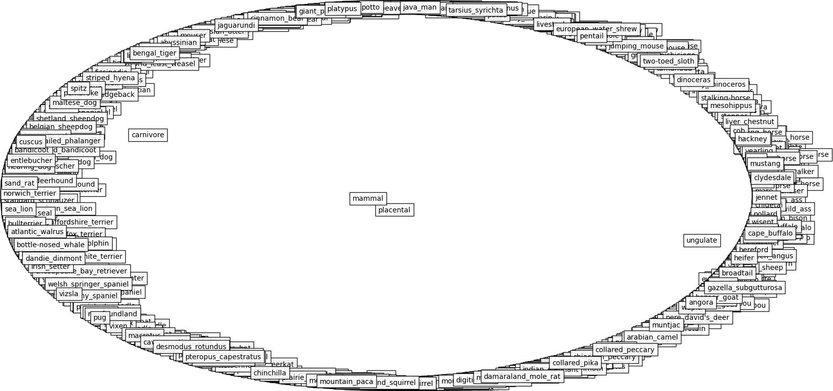
WordNet mammals has a low Gromov hyperbolicity.

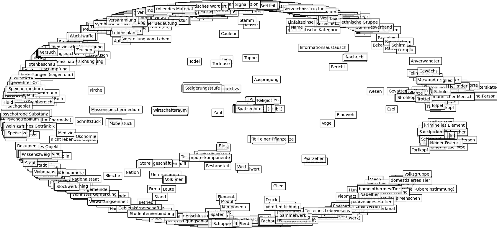
I also tried the dataset OpenThesaurus which has a pretty high Gromov hyperbolicity. It is a German dataset, but even if you don’t understand this language, you should see the difference.

Applications

Besides visualizations, various uses can be found for these embeddings:

• clustering with hyperbolic k-means
• finding wrong relations in graphs [3]
• hypernym-hyponym detection [4]
• inside another network for other applications
• …

However, if you need word similarity or analogy there are better word embeddings. For example, SGNS (skip-gram with negative-sampling) produces quite good results for these tasks.

References

[1] M. Nickel and D. Kiela, Poincaré Embeddings for Learning Hierarchical Representations, 2017.

[2] M. Nickel and D. Kiela, Learning Continuous Hierarchies in the Lorentz Model of Hyperbolic Geometry, 2018.

[3] S. Roller, D. Kiela and M. Nickel, Hearst Patterns Revisited: Automatic Hypernym Detection from Large Text Corpora, 2018.

[4] M. Le, S. Roller, L. Papaxanthos, D. Kiela and M. Nickel, Inferring Concept Hierarchies from Text Corpora via Hyperbolic Embeddings, 2019.