Metrics for uncertainty estimation

07 Aug 2020

Predictions are not just about accuracy, but also about probability. In lots of applications it is important to know how sure a neural network is of a prediction. However, the softmax probabilities in neural networks are not always calibrated and don’t necessarily measure uncertainty.

In this blog post, I will implement the most common metrics to evaluate the output probabilities of neural networks.

There are in general two types of metrics:

1. Proper scoring rules estimate the deviation from the true probability distribution. A high value indicates that the predicted probability \(0 \leq \hat{p} \leq 1\) is far away from the true probability \(p \in \{0, 1\}\). Whether \(\hat{p}\) equals \(0.6\) or \(\hat{p}\) equals \(0.8\) is not as important as the distance from \(1\) or \(0\).
2. Calibration metrics measure the difference between “true confidence” and “predicted confidence”. If \(\hat{p}\) equals \(0.6\), then it should mean that the neural network is 60% sure. A model is calibrated if \(\mathbf{P}\left(\hat{Y} = y \mid \hat{P} = p\right) = p\). Then the difference is \(\left\lvert \mathbf{P}\left(\hat{Y} = y \mid \hat{P} = p\right) - p\right\rvert\). The predicted confidence is the output probability of the neural network, while the true confidence is estimated by the corresponding accuracy. Calibration metrics are computed on the whole dataset in order to group different probabilities (e.g. 0% - 10%, 10% - 20%, …). In contrast, proper scoring rules compare individual probabilities.

14/08/20 update: added recommendations, static calibration error and thresholding

30/08/21 update: the traditional reliability diagram, as it is known from weather forecasts, has the relative frequency and not the accuracy on the y-axis. However, papers like “On Calibration of Modern Neural Networks” have the accuracy on the y-axis. I use the latter convention here but would recommend the traditional definition as it gives better results.

Proper scoring rules

Negative log likelihood

Negative log likelihood (NLL) is the usual method for optimizing neural networks for classification tasks. However, this loss function can also be used as a uncertainty metric. For example, the Deepfake Detection Challenge scored submissions on NLL.

where \(p_j = 1\) is the ground truth and \(\hat{p}_j = \text{softmax}_j\left(x\right)\). PyTorch’s CrossEntropyLoss applies the softmax function and computes \(H(p, \hat{p})\).

import torch.nn as nn

loss_func = nn.CrossEntropyLoss(reduction="mean")
nll = loss_func(logits, target)

We can also rewrite the code above using nll_loss. This shows more of what happens internally.

import torch
import torch.nn.functional as F

logits = torch.exp(logits - torch.max(logits, dim=-1, keepdim=True))
pred = torch.log(logits) - torch.log(torch.sum(logits, dim=-1, keepdim=True))
nll = F.nll_loss(pred, target, reduction="mean")

To ensure numerical stability \(\max(x)\) was subtracted from \(\log\left(\text{softmax}_j\left(x\right)\right)\).

Brier score

The Brier score is the mean squared error of a forecast. For a single output it is defined as follows:

For multiple values it is possible to sum over all outputs. The code is then

def brier_score(y_true, y_pred):
  return 1 + (np.sum(y_pred ** 2) - 2 * np.sum(y_pred[np.arange(y_pred.shape[0]), y_true])) / y_true.shape[0]

y_true should be a one dimensional array, while y_pred should be a two dimensional array. When predicting multiple classes, sometimes each class is considered individually (one-vs.-rest / one-against-all strategy).

Calibration metrics

Expected calibration error

We approximate the probability distribution by a histogram with \(B\) bins. Then \(\mathbf{P}(\hat{P} = p) = \frac{n_b}{N}\) where \(n_b\) is the number of probabilities in bin \(b\) and \(N\) is the size of the dataset. Since we put \(n_b\) probabilities into one bin, \(p\) is not a single value. Therefore, a representative value \(p = \sum_{\hat{p_i} \in b} \frac{\hat{p_i}}{n_b} = \text{conf}(b)\) is necessary. Similarly, we can set \(\mathbf{P}(\hat{Y} = y \mid \hat{P} = p) = \sum_{\hat{y}_i \in b} \frac{\mathbf{1}\left(y_i = \hat{y_i}\right)}{n_b} = \text{acc}(b)\) where \(\hat{y_i}\) is obtained from the highest probability (arg max). \(\hat{p_i}\) is also the highest probability (max).

ECE is then defined as follows:

The accuracy \(\text{acc}(b)\) is also called “observed relative frequency”, while the confidence \(\text{conf}(b)\) is a synonym for “average predicted frequency”.

The implementation is:

def expected_calibration_error(y_true, y_pred, num_bins=15):
  pred_y = np.argmax(y_pred, axis=-1)
  correct = (pred_y == y_true).astype(np.float32)
  prob_y = np.max(y_pred, axis=-1)

  b = np.linspace(start=0, stop=1.0, num=num_bins)
  bins = np.digitize(prob_y, bins=b, right=True)

  o = 0
  for b in range(num_bins):
    mask = bins == b
    if np.any(mask):
        o += np.abs(np.sum(correct[mask] - prob_y[mask]))

  return o / y_pred.shape[0]

y_true should be a one dimensional array like np.array([0,1,0,1,0,0]), while y_pred requires a two dimensional array e.g. np.array([[0.9, 0.1],[0.1, 0.9],[0.4, 0.6],[0.6, 0.4]], dtype=np.float32). Since most papers use between 10 and 20 bins [1], I set num_bins=15. More bins reduce the bias, but increase the variance (bias-variance tradeoff).

If you have TensorFlow Probability installed, you can also use the following function (which produces the same results):

import tensorflow_probability as tfp

tfp.stats.expected_calibration_error(num_bins=15, labels_true=gt, logits=np.log(pred))

Note if pred are logits, then np.log is not necessary.

There are a few problems with the standard ECE. np.linspace will create evenly spaced bins, which are likely to be empty. In statistics, bins are often chosen so that each bin contains an equal number of probability outcomes [2]. This is called Adaptive Calibration Error (ACE) in [1].

One can change the variable b in expected_calibration_error to obtain ACE.

b = np.linspace(start=0, stop=1.0, num=num_bins)
b = np.quantile(prob_y, b)
b = np.unique(b)
num_bins = len(b)

However, the adaptivity can also cause the number of bins to decrease. At the start of a neural network I trained, there were \(15\) bins. After 10 epochs the number of bins reduced to \(11\). The sigmoid function tends to over-emphasize probabilities near \(1\) or \(0\). For example, one training run produced the bins \(\{0.4786461, 0.99776319, 0.99977307, \dots, 0.99995485, 0.99999988, 1., 1.\}\).

It is also important to note that only the highest probability is considered for ECE/ACE i.e. pred_y = np.argmax(y_pred, axis=-1). [2] proposes Static Calibration Error (SCE) which bins the predictions separately for each class probability. This should be considered, when all probabilities in a multi-class setting are equally important.

The implementation is:

def static_calibration_error(y_true, y_pred, num_bins=15):
  classes = y_pred.shape[-1]

  o = 0
  for cur_class in range(classes):
      correct = (cur_class == y_true).astype(np.float32)
      prob_y = y_pred[..., cur_class]

      b = np.linspace(start=0, stop=1.0, num=num_bins)
      bins = np.digitize(prob_y, bins=b, right=True)

      for b in range(num_bins):
        mask = bins == b
        if np.any(mask):
            o += np.abs(np.sum(correct[mask] - prob_y[mask]))

  return o / (y_pred.shape[0] * classes)

If there are a lot of classes, adaptive SCE will assign too many bins to predictions close to 0% (e.g. 999 classes \(\approx 0.01\), 1 class \(\approx 0.99\)). ECE does not have the same problem, because it only evaluates the class with the highest probability. [1] suggests thresholding the predictions in this case (e.g. \(10^{-3}\)). Change the code as follows:

...
prob_y = y_pred[..., cur_class]
mask = prob_y > threshold
correct = correct[mask]
prob_y = prob_y[mask]
...
o += np.abs(np.sum(correct[mask] - prob_y[mask])) / prob_y.shape[0]
...
return o / classes

Some other things to keep in mind are:

• optimizing ECE: using scipy.optimize it is possible to directly optimize this non-differentiable metric. However, according to [1] “ECE is very strongly influenced by measures of calibration error that adhere to its own properties, rather than capturing a more general concept of the calibration error.”
• norm: most paper use the \(L_1\) norm, but \(L_2\) is also an option.

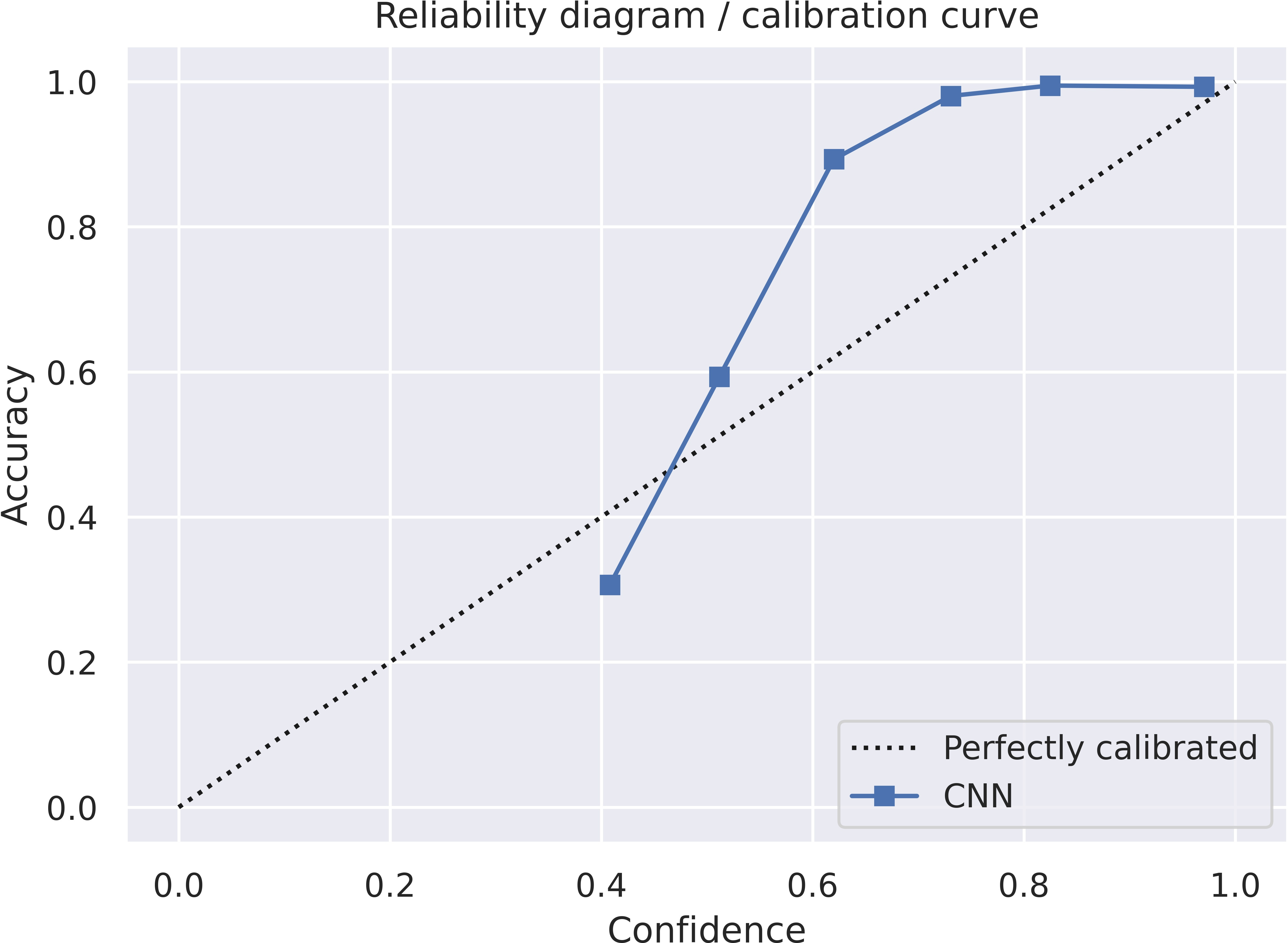
Reliability diagram

The x-axis is np.sum(prob_y[mask]) / count (confidence or avg predicted frequency) and the y-axis is np.sum(correct[mask]) / count) (accuracy). It is important to note that the traditional reliability diagram has on the y-axis the “observed relative frequency” np.sum(y_true[mask]) / count) and NOT the accuracy. I would also recommend using the “observed relative frequency” as this is the standard approach.

First, we change the function expected_calibration_error to return both values. Then the following function will produce a reliability diagram:

import matplotlib.pyplot as plt
import seaborn as sns

sns.set()

def reliability_diagram(y_true, y_pred):
    x, y = expected_calibration_error(y_true, y_pred)

    plt.plot([0, 1], [0, 1], "k:", label="Perfectly calibrated")
    plt.plot(x, y, "s-", label="CNN")

    plt.xlabel("Confidence")
    plt.ylabel("Accuracy")
    plt.legend(loc="lower right")
    plt.title("Reliability diagram / calibration curve")

    plt.tight_layout()
    plt.show()

The reliability diagram itself looks like this:

Recommendations

Using an unsuitable metric can lead to wrong conclusions. According to [3], calibration metrics should not be used to compare different models. Expected calibration error is sensitive to the number of bins and the thresholding. Furthermore, it does not provide a consistent ranking of different models.

Instead, a better metric would be BS and log likelihood provided temperature scaling was applied to the logit layer. ECE is more useful for measuring the calibration of a specific model.

References

[1] J. Nixon, M. Dusenberry et al., Measuring Calibration in Deep Learning, 2020.

[2] Hyukjun Gweon and Hao Yu, How reliable is your reliability diagram?, 2019.

[3] A. Ashuskha, A. Lyzhov, D. Molchanov et al. Pitfalls of in-domain uncertainty estimation and ensembling in deep learning, 2020.